CS7641 Project : Machine Learning on PM2.5 pattern variation

1 Introduction/Background:

Air pollution, especially suspended particulate matter (PM) pollution, has been significantly mitigated in China over the past 10 years through continuous government emission regulation efforts. However, the specific achievements have varied from city to city due to the complex influences of emission reduction, atmospheric chemistry regimes, regional characteristics, and meteorological patterns.

A dominant fraction of PM2.5 particles are secondarily formed in the atmosphere, with volatile organic compounds (VOCs) such as toluene and isoprene as the primary precursors. VOCs are predominantly of biogenic origin (BVOCs) at a global scale, while anthropogenic sources (AVOCs) can also dominate in densely populated cities. The formation of PM2.5 involves a multitude of complex atmospheric chemical reactions, with oxidants species and nitrogen oxides playing a central role.

2 Problem Definition

In this project, we collected hourly in situ measurements of fine particulate matter (PM2.5) mass concentration in 317 cities across China from 2015 to 2023 from China National Environmental Monitoring Center (CNEMC, https://quotsoft.net/air/). We would compile an extensive dataset, including BVOC emissions inventories from CAMS global emission inventories(https://ads.atmosphere.copernicus.eu/), AVOC emissions from the Multi-resolution Emission Inventory model for Climate and air pollution research (http://meicmodel.org.cn/), gas pollutant concentrations from CNEMC, and meteorological fields from ECMWF Reanalysis v5 (https://www.ecmwf.int/en/forecasts/dataset/ecmwf-reanalysis-v5) data. These features represent the central factors that impact the PM2.5 pollution, i.e., precursor concentration, atmospheric chemistry regime, meteorological transfer.

The main objectives of this project are:

1. Analyze the primary factors contributing to the reduction in PM2.5 concentrations in China over the past ten years and evaluate the effectiveness of air pollutant emission reduction regulation.

2. Investigate the seasonal variation patterns of PM2.5 concentrations in different cities and identify potential pattern change with time.

3. Identify the regional patterns by clustering different cities regarding of PM2.5 concentration trend and seasonal variation patterns.

3 Methods

3.1 Data collection and preprocessing

We first processed the hourly PM2.5 concentration data to daily average and only used days with at least 17 hours of data. We further derived the monthly and annual mean from the daily averages.

3.2 Unsupervised method: K-means clustering

Here we used L2 norm to conduct clustering, i.e., the Euclidean distance was used. We didn’t use Dynamic Time Warping (DTW) although DTW is a similarity measure between time series. This is because our temperal profilesare synchronous which doesn’t allow for stretching and translation.

3.2.1 Annual mean trend

We firstly clustered the 9-year annual mean trends for 317 cities using K-mean clustering. The annual mean PM2.5 concentrations are normalized for each city by

3.2.2 Seasonal trend based on monthly trend

We further clustered the seasonal trends for 317 cities using K-mean clustering. The seasonal trend component of the 9-year PM2.5 temperal profiles for each city was derived following this webpage.

In brief, the total monthly temperal variations were expressed as the summation of long-term trend, seasonal trend and residuals. The long-term trend was fitted using a polynomial function.

The cluster numbers were determined based on the distortion elbow figure (distortion vs. cluster numbers), as shown in Fig. 1a and 1d. Ultimately, we generated three clusters for the annual mean trend and four clusters for the seasonal trend. We evaluated our clustering results using the Silhouette Coefficient (Fig. 1b and 1e) and the Davies-Bouldin Index (Fig. 1c and 1f). The Silhouette Coefficients were greater than 0.2 for both clustering scenarios. Considering the ratio of feature numbers to sample numbers (9 vs. 317) and the dispersion level of our data, our clustering results are acceptable.

3.3 Supervised method:

We will also use features or factors including VOCs emission, chemistry indicator and meteorological parameters to train a prediction model to predict the PM2.5 temporal profiles and seasonal variation patterns. For the prediction model, we will use both tree-based method and artificial neural network. For the tree-based method, we will choose to use the gradient boosted tree method. For the artificial neural network, we will used the long-term memory structure. These methods are known to be effective on the time series prediction. Here is the list of the methods and functions we used/plan to use in this project:

Method	Libraries	Function
K-mean	scikit-learn	sklearn.cluster.KMeans
Gradient Boost Tree Method	XGBoost	XGBoost.XGBRegressor
Random Forest Regressor	scikit-learn	sklearn.ensemble.RandomForestRegressor

4 Results and Discussion

4.1 K-mean clustering results

4.1.1 Annual trend

We generated two main clusters from the annual PM2.5 trends of 317 cities, with a third cluster representing outliers that could not be represented by the two main clusters. The annual trends for each cluster center are shown in Fig. 2a-c, while Fig. 2d displays the spatial distribution of the clustering results for all 317 cities. For cities in Cluster 1, PM2.5 mass concentration declined continuously from 2014 to 2022, due to persistent emission reduction measures implemented by the Chinese government. However, there was a rebound in PM2.5 concentrations in 2023 for these cities. Cluster 1 includes most of the cities in the provinces of Heilongjiang, Jilin, Liaoning, Beijing, Hebei, Shandong, Henan, Hunan, Hubei, Zhejiang, Sichuan, Chongqing, Tibet, Ningxia, and Qinghai.

In contrast, cities in Cluster 2 showed a decline in PM2.5 concentration only after 2017, with a similar rebound in 2023. The delayed decrease in PM2.5 concentration for Cluster 2 might be related to different chemistry regimes, pollutant emission structures and delayed implementation of emission reduction practices in provinces such as Shanxi, Jiangsu, Anhui, and many southern provinces.

The remaining cities in Cluster 3 (outliers) did not show a clear decrease in PM2.5 concentration over the past nine years, particularly evident in many cities in Yunnan province. Overall, the annual trends for PM2.5 concentrations in 317 cities in China showed distinct spatial patterns from 2014 to 2023. Further investigation into the reasons for this phenomenon will be discussed in supervised model section.

4.1.2 Seasonal trend

Figure 3 shows the seasonal trends for each cluster center and the spatial distribution of each cluster. For Cluster 1, PM2.5 mass concentration decreased from January to August and increased after August. For Cluster 2, PM2.5 concentration peaked in March and reached its lowest levels from June to August. For Cluster 3, the highest PM2.5 concentration was found in January, while the lowest concentrations were in July and August. For Cluster 4, PM2.5 concentration peaked in December and January and reached its lowest in June.

These four clusters exhibit distinct spatial patterns. Cluster 3 includes most of the cities in central China and Xinjiang. Cluster 4 encompasses cities in southern China, mainly in Hainan, Guangdong, Guangxi, Jiangxi, and Fujian provinces. Cluster 2 includes cities in Yunnan province and several coastal cities in Fujian province. Cluster 1 represents most of the cities in northeastern, northwestern China, and Jiangsu province.

The different seasonal patterns reflect varying meteorological conditions, emission structures, and chemical regimes across different regions, which will be further addressed in the supervised model section.

4.2 Supervised Results

We then trained a supervised model with the monthly average of PM2.5 concentration, meteorological variables, and emissions. The variables we considered are listed below.

Full Name	Unit	Short Name
u wind at 10m	m/s	u10
v wind at 10m	m/s	v10
Dewpoint at 2m	K	d2m
Temperature at 2m	K	t2m
Boundary Layer Height	m	blh
Cloud Base Height	0 - 1	cbh
Surface Pressure	Pa	sp
Shortwave Solor downward radiation	J m**-2	ssrd
Total Cloud Cover	0 - 1	tcc
Total Cloud Ice Water Content	kg m**-2	tciw
Total Cloud Liquid Water Content	kg m**-2	tclw
Total Precipitation	m	tp
UV visible albedo for diffuse radiation	0 - 1	aluvd
UV visible albedo for direct radiation	0 - 1	aluvp
Formaldehyde Column Concentration	molec/cm2	HCHO_col
Alpha Pinene Emission	kg/m2/s	alpha-pinene
Beta Pinene Emission	kg/m2/s	beta-pinene
Isoprene Emission	kg/m2/s	isoprene
Monoterpenes Emission	kg/m2/s	other-monoterpenes
sesquiterpenes Emission	kg/m2/s	sesquiterpenes
Black Carbon Anthropogenic Emission	kg/km2/yr	BC
CO Anthropogenic Emission	kg/km2/yr	CO
Ammonia Anthropogenic Emission	kg/km2/yr	NH3
NOx Anthropogenic Emission	kg/km2/yr	NOx
PM25 Anthropogenic Emission	kg/km2/yr	PM25
CH4 Anthropogenic Emission	kg/km2/yr	CH4
SO2 Anthropogenic Emission	kg/km2/yr	SO2
Nonmethane VOC Anthropogenic Emission	kg/km2/yr	VOC

We started by applying the unsupervised results to perform supervised predictions and found few differences in the results among the clusters. Therefore, we decided to train the model with the entire dataset for integration and robustness of the simulation results. Our hyperparameters were selected with cross-validation achieved by GridSearchCV from sklearn.

Figures 4 and 5 show the resulting predictions using Random Forest and XGBoost, respectively. Both models provide good forecasts, given their $R^2$ and $MAPE$ values. However, XGBoost performs slightly better compared to Random Forest. The better performance of XGBoost is partially due to its ability to handle missing data internally, as we only pruned sites with less than 5% data points of the whole study period; missing data points still exist in our training dataset. Additionally, XGBoost uses gradient descent to optimize the loss function, making it more efficient in finding the optimal splits in the trees and providing better statistical measures for model evaluation. It should be noted that both models showed poorer performance under extremely high PM2.5 conditions. This implies the complicated mechanism of the formation of extreme PM2.5 events, during which the relative contribution of independent factors is not uniform.

As shown in Figures 6 and 7, temperature and HCHO dominate local PM2.5 concentrations. The importance of other features is much smaller, which might explain the different orders of their relative importance given by the two models. The high sensitivity of PM2.5 to temperature suggests difficulties in air quality control under future climate changes, while the high impacts of HCHO highlight the importance of VOC emission controls in future air quality policies.

5 Next Step

We found the consistently distributed relative importance of features among the clusters. To further explain the notable cluster behaviors of PM2.5 temporal variations, we plan to investigate the time series of features based on the order of their relative importance. The clustering result based on seasonal variations approximately agrees with the climate zone distribution in China, suggesting that it might be beneficial for us to examine the time series of meteorological features, especially t2, given its significant contribution.

To sum up, we need to analyze the trends and seasonality of meteorological patterns as well as emission activity, and evaluate their roles in the observed clustering behaviors of PM2.5 concentrations in the cities.

Figures

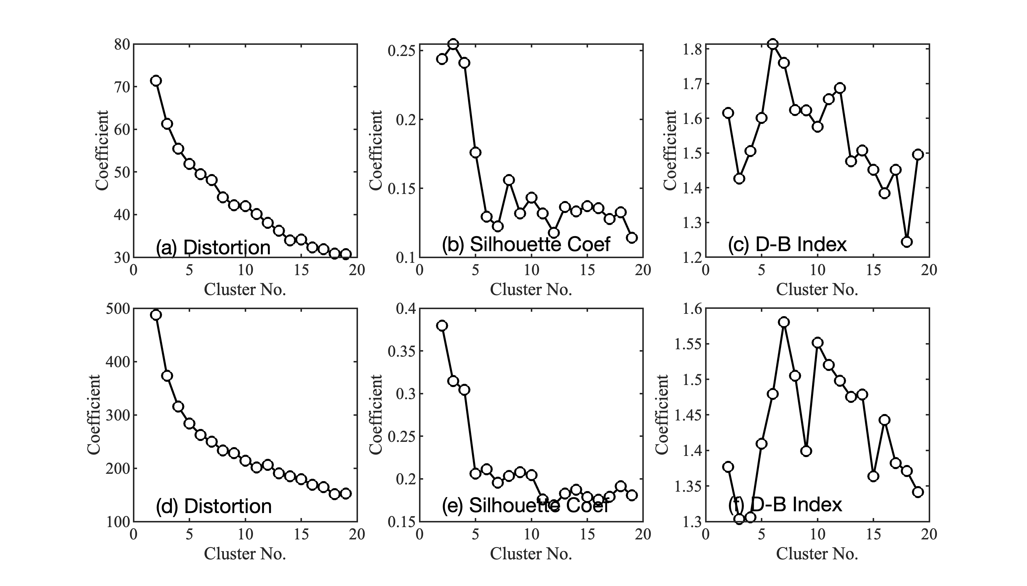Figure 1. Evaluation for K-mean clustering of PM2.5 concentration annual mean trend (a-c) and seasonal trend (d-f)

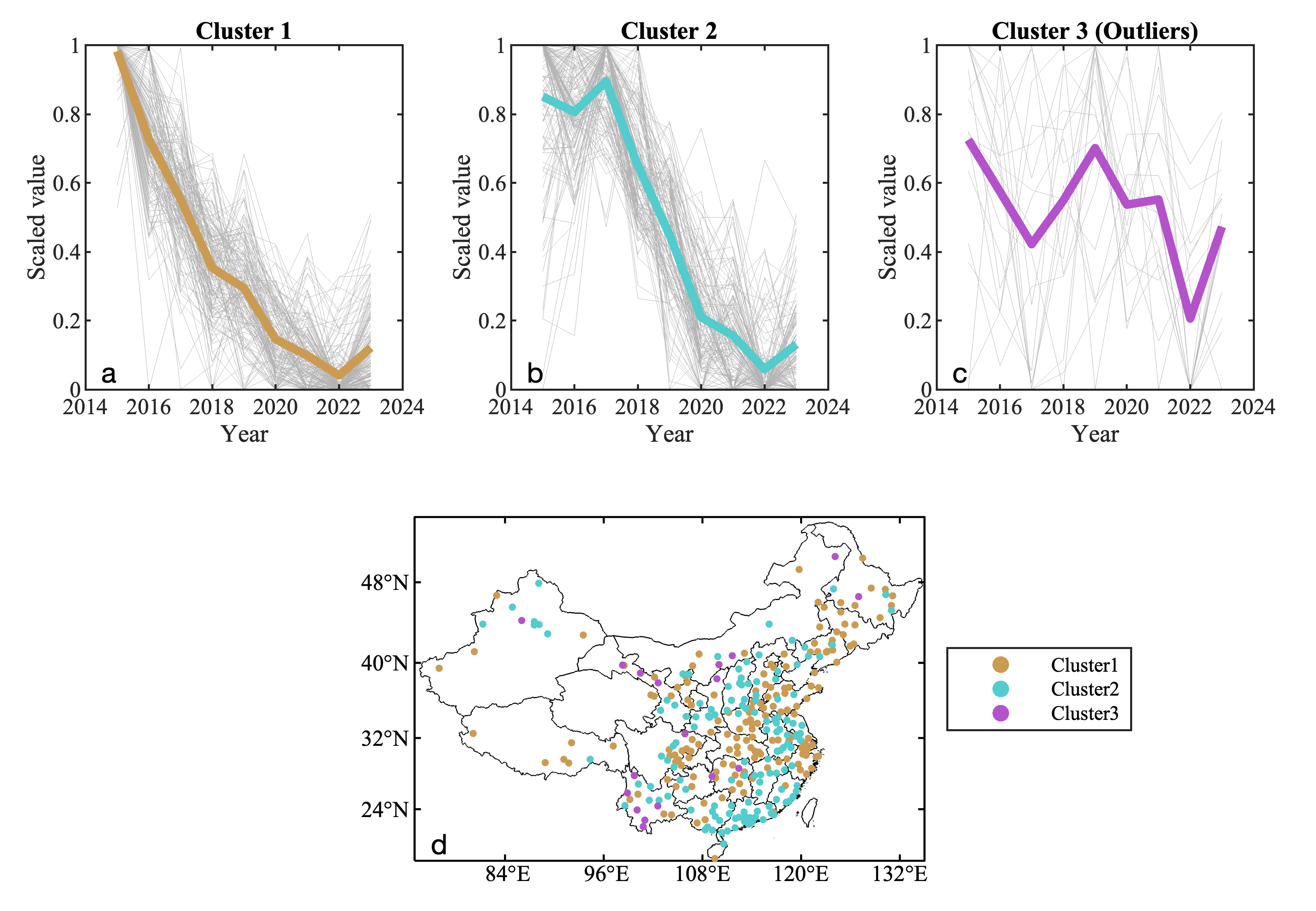Figure 2. PM2.5 concentration annual mean trend centers for each clusters (a-c) and spatial distribution of clustering results (d)

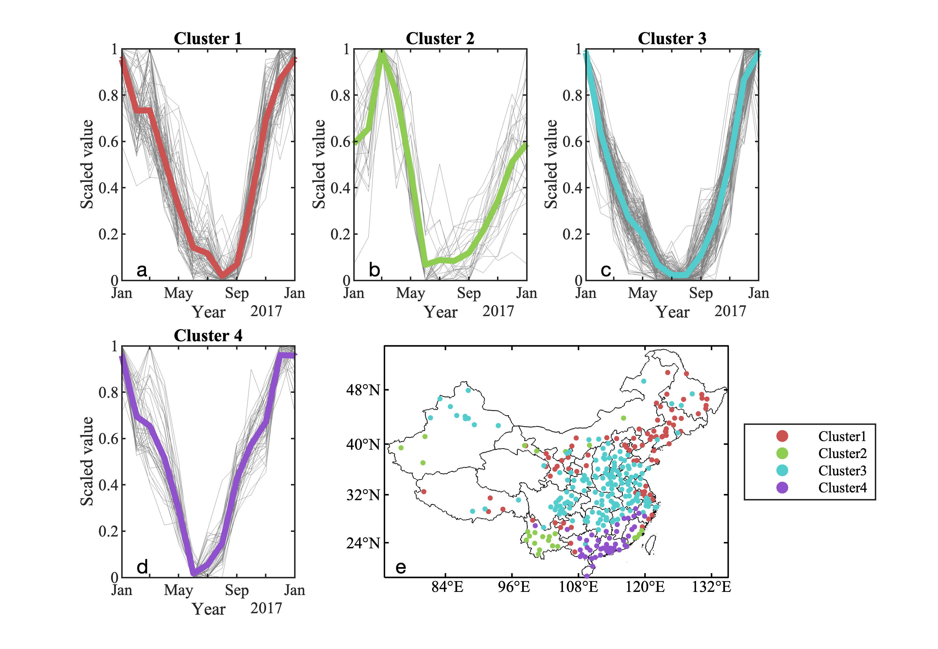Figure 3. PM2.5 concentration seasonal trend centers for each clusters (a-d) and spatial distribution of clustering results (e)

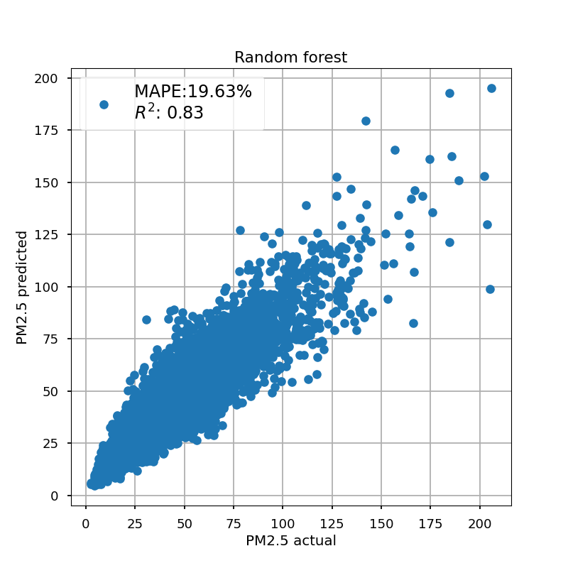
Figure 4. PM2.5 predicted with random forest

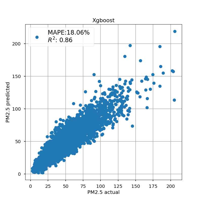
Figure 5. PM2.5 predicted with XGboost

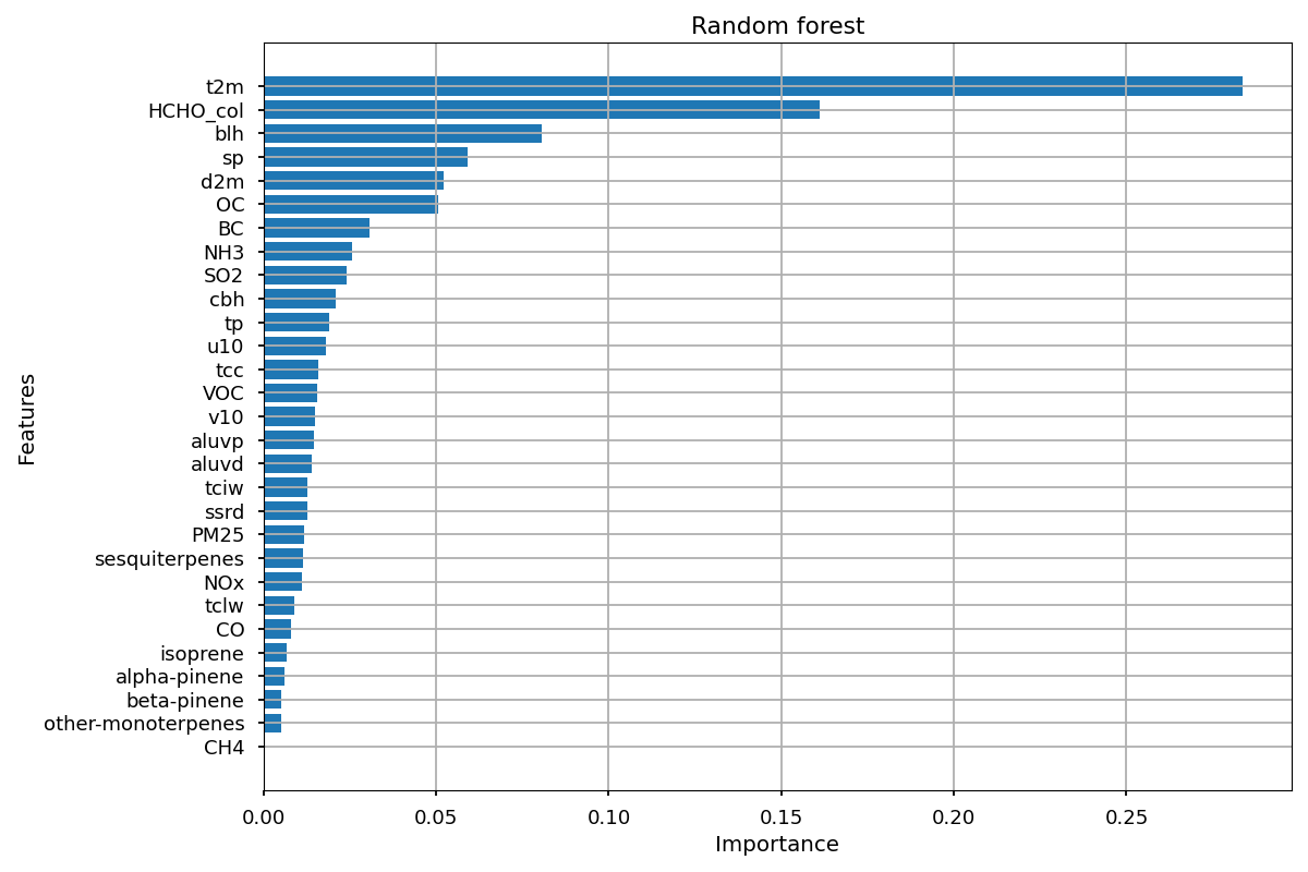
Figure 6. Feature importances based on Random Forest

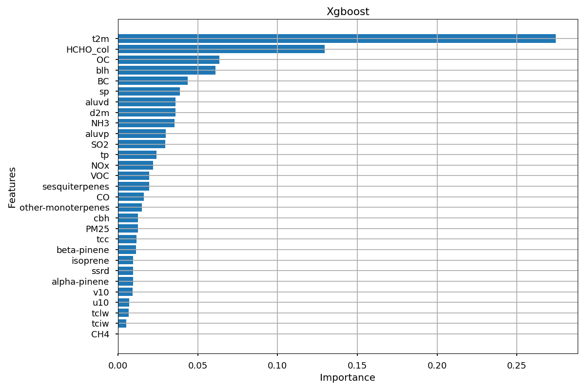
Figure 7. Feature importances based on XGBoost

References

1. Z. Ma, R. Liu, Y. Liu, and J. Bi, “Effects of air pollution control policies on PM2.5; pollution improvement in China from 2005 to 2017: a satellite-based perspective,” Atmospheric Chemistry and Physics, vol. 19, no. 10, pp. 6861-6877, 2019, doi: 10.5194/acp-19-6861-2019.

2. S. Guo et al., “Elucidating severe urban haze formation in China,” Proc Natl Acad Sci U S A, vol. 111, no. 49, pp. 17373-8, Dec 9 2014, doi: 10.1073/pnas.1419604111.

3. S. Zhao, D. Yin, Y. Yu, S. Kang, D. Qin, and L. Dong, “PM(2.5) and O(3) pollution during 2015-2019 over 367 Chinese cities: Spatiotemporal variations, meteorological and topographical impacts,” Environ Pollut, vol. 264, p. 114694, Sep 2020, doi: 10.1016/j.envpol.2020.114694.

4. R. J. Huang et al., “High secondary aerosol contribution to particulate pollution during haze events in China,” Nature, vol. 514, no. 7521, pp. 218-22, Oct 9 2014, doi: 10.1038/nature13774.

5. M. Shrivastava et al., “Recent advances in understanding secondary organic aerosol: Implications for global climate forcing,” Reviews of Geophysics, vol. 55, no. 2, pp. 509-559, 2017, doi: 10.1002/2016rg000540.

6. Z. Wu et al., “Aerosol Liquid Water Driven by Anthropogenic Inorganic Salts: Implying Its Key Role in Haze Formation over the North China Plain,” Environmental Science & Technology Letters, vol. 5, no. 3, pp. 160-166, 2018, doi: 10.1021/acs.estlett.8b00021.

Final Contributions

Name	Contribution
Bin Bai	Data Preprocessing & Model Train & Result Discussions & Video
Fanghe Zhao	Data Preprocessing & Model Train & Result Discussions& Report Writting
Shengjun Xi	Data Preprocessing & Result Discussions & Report Writting